Long story short
“is an area of machine learning concerned with how software agents ought to take actions in an environment in order to maximize the notion of cumulative reward.“
Wikipedia
Do you remember news that a computer could fully beat the Mario Bros 🍄 game? That’s the technique which was used behind 🤗
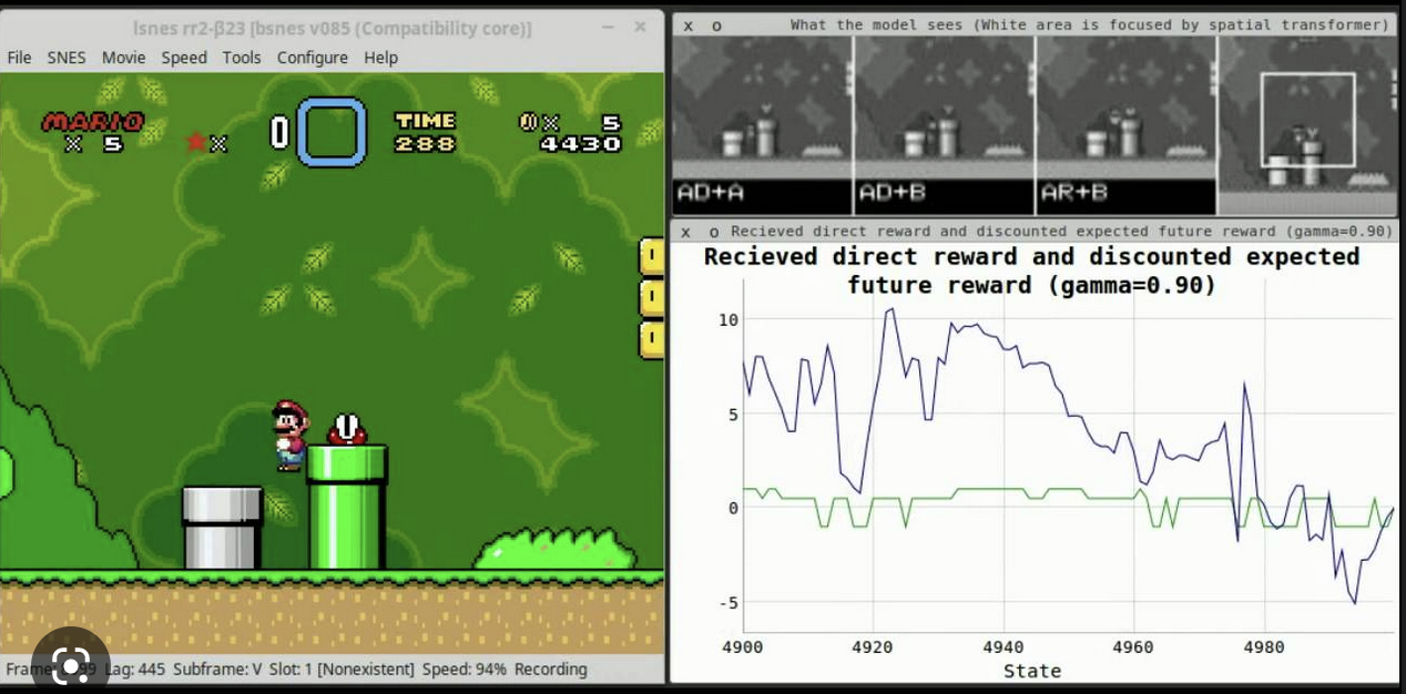
Table of contents
- Long story short
- Table of contents
- Introduction
- Reinforcement learning with deep neural networks
- Example implementation
- Summary
Introduction
What are main ideas behind it?
Reinforcement learning (RL) is a type of machine learning in which an agent learns to make decisions by interacting with its environment. The agent’s goal is to maximize a reward signal by choosing actions that will lead to the highest expected reward.
💡 Agent is a term known from, inter alias, computer simulations. It can be understood as an entity type, with coded some intelligence behind it, doing some work every iteration of the computer program.
The basic idea behind RL is to learn a policy, which is a mapping from states of the environment to actions. The policy defines the behavior of the agent, determining which action to take in each state. The agent interacts with the environment by selecting actions according to its current policy, and the environment responds by transitioning to a new state and providing a reward signal.
About Q-learning
The agent’s goal is to learn a policy that maximizes the expected cumulative reward over time, also called return. To do this, the agent uses a technique called Q-learning, which learns the optimal action-value function. The action-value function, denoted as Q(s, a), gives the expected return for taking action a in state s and then following the policy thereafter.
Bellman equation
The Q-learning algorithm updates the action-value function based on observed experiences, by using the Bellman equation which states that the optimal action-value function is the expected reward plus the discounted maximum action-value of the next state.
In addition to Q-learning, there are other RL methods such as SARSA, Deep-Q Network (DQN), Trust Region Policy Optimization (TRPO), Proximal Policy Optimization (PPO) and so on. The choice of algorithm depends on the problem and the specific requirements of the application.
Deep-Q Network tutorial can be found here: https://towardsdatascience.com/deep-q-learning-tutorial-mindqn-2a4c855abffc (although it’s not required passing it to continue with our Python examples)
Where is it used?
Reinforcement learning has been used to solve a wide variety of problems, including:
chess and Go,
controlling robots,
optimizing manufacturing processes,
and even – trading stocks.
It’s still an active research area with many open problems and challenges. Overall, RL is a powerful framework for learning optimal decision-making policies in complex, dynamic environments where the optimal solution is not known in advance and needs to be learned through trial and error.
Before going to the Python example, let’s mention the power of reconciling reinforcement learning and deep neural networks.
Reinforcement learning with deep neural networks
Reinforcement learning can be used in conjunction with deep neural networks. In fact, many recent successes in reinforcement learning have used deep neural networks to approximate the action-value function or the policy.
One popular approach is to use a deep neural network to approximate the Q-function in Q-learning. This is known as a Deep Q-Network (DQN). The neural network takes in the state of the environment as input and produces a vector of Q-values, one for each possible action. The Q-values are then used to select the action with the highest expected return. The neural network is trained to minimize the difference between the predicted Q-values and the true Q-values, as determined by the Q-learning algorithm.
Another approach is to use a deep neural network to directly represent the policy, without using a separate Q-function. This approach is known as policy gradient methods and one of the popular variant is the Proximal Policy Optimization (PPO). The neural network takes in the state of the environment as input and produces a probability distribution over actions. The agent selects actions according to the probability distribution and the network is trained to maximize the expected return.
These methods have been used to achieve state-of-the-art performance in a wide range of RL tasks, such as playing Atari games, Go, and even complex 3D environments like the Dota 2, FPS games, and so on.
In summary, deep neural networks can be used in reinforcement learning as a powerful tool to approximate the Q-function or policy and they are widely used to improve the performance of the algorithms and to handle more complex and high dimensional environments.
Example implementation
Prerequisite
You’ll be needing a Python interpreter, optionally jupyter-lab set up, and the example data (labyrinth). All can be found on my GitHub here: https://github.com/PuzzleLearning/rf-labyrinth
Solving the labyrinth
We’ll go through an example of how reinforcement learning can be used to solve a labyrinth using the Q-learning algorithm in Python.
First, we need to define our environment. That is, we start with the binary definition of the labyrinth.
import numpy as np

# Define the labyrinth
labyrinth = np.array([
    [0, 0, 0, 0, 0],
    [0, 1, 0, 1, 0],
    [0, 1, 0, 1, 0],
    [0, 1, 0, 1, 0],
    [0, 0, 0, 0, 0]
])
# Define the Q-table
q_table = np.zeros((labyrinth.shape[0], labyrinth.shape[1], len(actions)))
Agent needs to know “what to do”, so let’s define a set of possible actions:
# Define the possible actions
actions = ["up", "down", "left", "right"]
Next, let’s define some parameters of our simulation:
# Define the learning rate
alpha = 0.8

# Define the discount factor
gamma = 0.95

# Define the exploration rate
epsilon = 0.1

# Define the maximum number of episodes
episodes = 10000
Let’s focus now on the code of our simulation – this is the place were the RF learning will take place in an iterative manner.
# Train the Q-learning algorithm
for episode in range(episodes):
    # Set the initial state
    state = (0, 0)

    # Loop until the agent reaches the goal
    while True:
        # Select the action with the highest Q-value
        if np.random.uniform(0, 1) < epsilon:
            action = np.random.choice(actions)
        else:
            action = actions[np.argmax(q_table[state[0], state[1]])]

        # Take the action and observe the new state and reward
        if action == "up":
            new_state = (state[0] - 1, state[1])
            reward = -1 if labyrinth[new_state[0], new_state[1]] == 1 else 0
        elif action == "down":
            new_state = (state[0] + 1, state[1])
            reward = -1 if labyrinth[new_state[0], new_state[1]] == 1 else 0
        elif action == "left":
            new_state = (state[0], state[1] - 1)
            reward = -1 if labyrinth[new_state[0], new_state[1]] == 1 else 0
        elif action == "right":
            new_state = (state[0], state[1] + 1)
            reward = -1 if labyrinth[new_state[0], new_state[1]] == 1 else 0

        # Update the Q-value
        q_table[state[0], state[1], actions.index(action)] = q_table[state[0], state[1], actions.index(action)] + alpha * (reward + gamma * np.max(q_table[new_state[0], new_state[1]]) - q_table[state[0], state[1], actions.index(action)])

        # Update the state
        state = new_state

        # Check if the goal is reached
        if state == (labyrinth.shape[0] - 1, labyrinth.shape[1] - 1):
            break
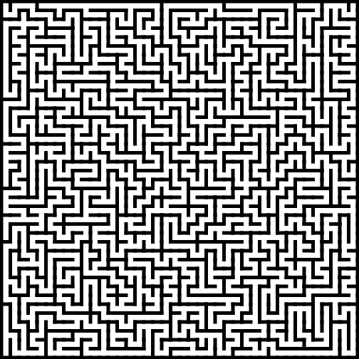
Advanced – labyrinth from a picture
It is possible to use reinforcement learning to solve a labyrinth represented in an image. One approach would be to use image processing techniques to extract information about the labyrinth from the image and then use that information as the input for the Q-learning algorithm.
Here is an example of how to use the Python OpenCV library to load an image of a labyrinth and extract the information needed to use it with Q-learning algorithm. We’ll be using picture of the maze, which was generated by a labyrinth generator.
[insert code here]This example reads an image of a labyrinth using the OpenCV library, and then uses the image to extract information about the labyrinth by converting the image to grayscale and applying a threshold to create a binary image. The position of the start and goal are found by scanning through the binary image, and then using this information to initialize the Q-table. The Q-learning algorithm is then used to train the agent to navigate the labyrinth.
Please keep in mind that this is just one way of how to approach solving labyrinth with reinforcement learning and image processing. The image pre-processing can be improved and the structure of Q-table, states, actions and rewards should be adjusted to the specific task at hand. Also depending on the size and complexity of the labyrinth, it might be not be efficient to store the Q-table in memory as it will be very large. In such cases, function approximates like neural networks could be used to approximate Q-values.
It is important to note that this example is an oversimplification of the problem, real-world images might have noise, lighting variations and other complexities that might need to be pre-processed, also the agent might get stuck in loops or never reach the goal due to poor exploration. These are all important things that need to be considered when working with real-world images.
Additionally, this example assumes that the labyrinth is represented in the image as white spaces (or 255 in grayscale) and walls are represented as black spaces (or 0 in grayscale). This may not be the case in all labyrinth images and the threshold value might need to be adjusted accordingly.
Summary
- Reinforcement learning is a method for training agents to make decisions in complex, dynamic environments by maximizing a reward signal.
- Q-learning is a popular RL algorithm that learns the optimal action-value function, which gives the expected return for taking a specific action in a specific state.
- Deep neural networks can be used to approximate the Q-function or policy in RL, which can improve performance and handle more complex environments.
- RL can be used to solve a wide variety of problems such as playing games, controlling robots, and optimizing manufacturing processes.
- RL technique can be used in combination with image processing to solve problems like finding a path in a labyrinth represented in an image.

You must be logged in to post a comment.